Why a Short Factory Power Spike May Not Equal a Demand-Charge Peak
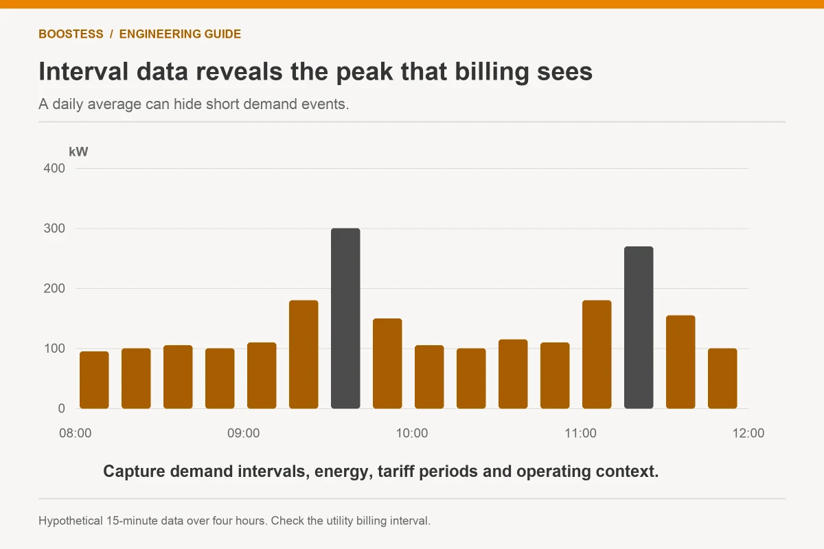
A short factory power spike may contribute very little to a billed demand peak when the tariff uses an averaged interval. Battery dispatch should therefore follow the actual meter calculation and commercial objective. The largest instantaneous number on a dashboard is not necessarily the number that sets the monthly demand charge.
This distinction changes both sizing and control. A brief motor event can require high instantaneous support but little energy. A modest load increase lasting throughout the billing interval can require more energy and have a larger billing effect. The following examples are hypothetical and use an assumed fifteen-minute averaging interval. Factories must verify their own tariff, meter timing and connection limits before applying the method.
Key Takeaways
- Reconstruct the billing calculation before sizing storage for demand reduction.
- Keep instantaneous connection limits separate from averaged billing demand.
- Test repeated peaks, charging recovery and tariff ratchets in the dispatch model.
On this page
- Obtain the rule behind the meter reading
- A one-minute spike and a fifteen-minute plateau
- The control target can change the battery requirement
- Avoid controllers that chase the wrong peak
- Recharge and ratchets can change the commercial result
- Make acceptance data resemble billing data
- Questions the buyer should ask
Obtain the rule behind the meter reading
Ask for the tariff version and metering definition that apply to the site. Determine whether demand uses fixed blocks, a rolling average, another calculation or a separate contracted-capacity rule. Record time-of-use periods, billing dates and any historical ratchet that can influence the billed value. These details vary by utility and contract.
Keep the measurement boundary explicit. A battery controller may read the main connection, a process feeder or its own inverter. Only the relevant connection measurement shows whether dispatch changes the utility’s demand figure. Feeder measurements help explain the event, but they need to reconcile with the billing boundary.
Align timestamps and interval start times. A factory historian and a utility meter may divide the same event differently if their clocks or interval boundaries differ. Obtain downloadable meter data where available and document the time zone, clock source and treatment of missing records. A visually similar daily curve is not enough for reconciliation.
NLR REopt supports evaluating site energy resources against economic objectives. For a demand-charge project, that evaluation requires the correct tariff structure and load data. The existing demand-charge guide explains the broad mechanism; the procurement study should go further and reproduce the site’s actual calculation.
A one-minute spike and a fifteen-minute plateau
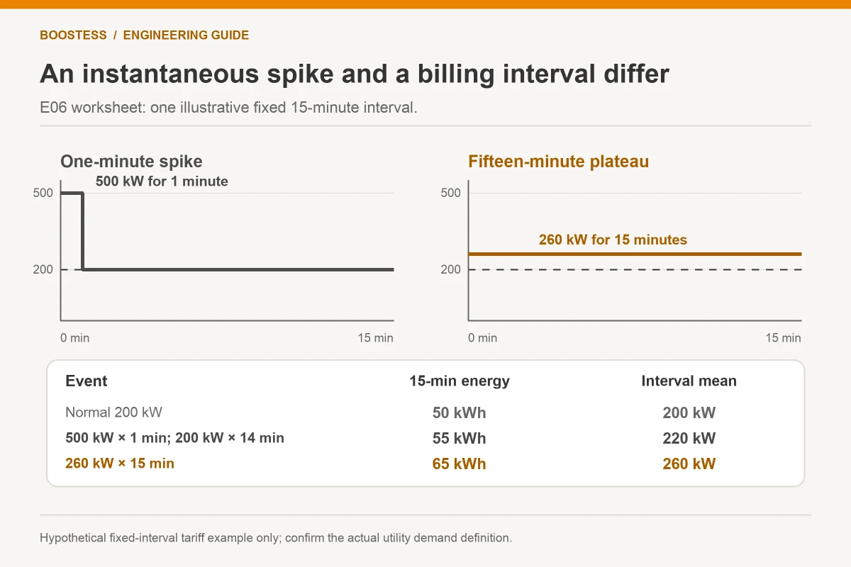
Assume a hypothetical fixed fifteen-minute interval. The factory normally consumes 200 kW. A process event raises demand to 500 kW for one minute, then load returns to 200 kW for the remaining fourteen minutes. Interval energy is 55 kWh: the first minute contributes about 8.33 kWh and the remaining time contributes about 46.67 kWh.
The average demand for that interval is 220 kW, calculated by dividing 55 kWh by one quarter of an hour. The 500 kW instantaneous spike raises this assumed billing interval by only 20 kW above the normal load. That does not mean the spike is irrelevant to electrical design; it means instantaneous and averaged objectives differ.
Now consider another event: the factory operates at 260 kW throughout all fifteen minutes. Its energy is 65 kWh and its interval demand is 260 kW. Although the instantaneous maximum is much lower than 500 kW, the assumed billed-demand effect is three times the first event’s 20 kW increase.
| Illustrative event | Maximum instantaneous load | Fifteen-minute energy | Assumed interval demand |
|---|---|---|---|
| Normal load | 200 kW | 50 kWh | 200 kW |
| One minute at 500 kW, then 200 kW | 500 kW | 55 kWh | 220 kW |
| Full interval at 260 kW | 260 kW | 65 kWh | 260 kW |
These examples use constant loads within their stated periods and exclude other site changes. They do not represent an actual utility bill. Use the same transparent method with measured data to identify which events deserve storage support.
The control target can change the battery requirement
To keep the one-minute event at an instantaneous ceiling of 200 kW, storage would need to supply 300 kW during the spike. That would require 5 kWh of delivered energy over one minute. Power is the demanding requirement in this version of the task.
If the objective were only to reduce the assumed fifteen-minute average from 220 kW to 200 kW, the battery would still need to deliver 5 kWh within the relevant interval. It might deliver that energy over a longer part of the interval at lower power, subject to the actual tariff, meter and controller design. Do not assume the two objectives require the same dispatch waveform.
For the 260 kW plateau, maintaining 200 kW through the whole interval would require 60 kW of discharge and 15 kWh of delivered energy. The lower instantaneous event now needs more energy. Repeating it six times without recharge would require 90 kWh before allowances.
The BOOSTESS brochure’s 105 kW / 241 kWh air-cooled cabinet gives a documented rated configuration to assess. Its nominal 105 kW output could fit the illustrative 60 kW plateau duty, subject to conditions and available energy. It would not supply the illustrative 300 kW instantaneous spike alone. Buying more battery energy within the same power rating does not resolve that gap.
Avoid controllers that chase the wrong peak
A controller responding to instantaneous power alone may discharge aggressively during a short spike and leave little reserve for a longer interval event. That strategy may suit a hard connection ceiling but perform poorly for a billing objective. The owner needs to specify which limit has priority.
For interval demand management, assess how the controller tracks energy accumulated within the current meter interval. It may use that information, load forecasts and remaining time to determine a dispatch target. Ask the supplier to explain the method and its limits in terms the owner can audit, without requiring disclosure of proprietary code.
Forecast error belongs in the test plan. A process assumed to stop in five minutes may continue for twenty. A control policy should show how it responds as the interval fills and reserve declines. Include actual production variation rather than modelling every shift as an identical curve.
Check the measurement response too. Sampling rate, communications delay, filtering and time alignment affect the controller’s view of a load event. No universal fast-response label establishes success against the site’s meter rule. The acceptance criterion should refer to the utility-defined calculation and separately to any instantaneous connection constraint.
Recharge and ratchets can change the commercial result
After discharge, storage charging becomes another site load. If the controller recharges while factory demand is already high, it can create a new peak and reverse part of the intended benefit. Define charging limits using the same connection boundary used for discharge.
The load-shifting versus peak-shaving discussion helps separate daily energy timing from demand control. In a factory with both objectives, test the combined schedule. Charging at an inexpensive energy rate is not automatically beneficial if it creates an expensive demand interval.
A tariff ratchet may also preserve part of a previously high demand charge. Verify the applicable formula and historical data before forecasting bill effects. Reducing the present month’s measured peak does not necessarily reduce the billed value by the same amount. Keep a tariff-specific calculation beside the physical dispatch model.
Where demand periods differ, simulate each period separately. One battery schedule may reduce an afternoon peak but raise a morning value. The financial model should retain these interactions rather than multiplying a single best-day reduction by every month of the year. Use transparent assumptions so that the owner can update the model when the tariff changes.
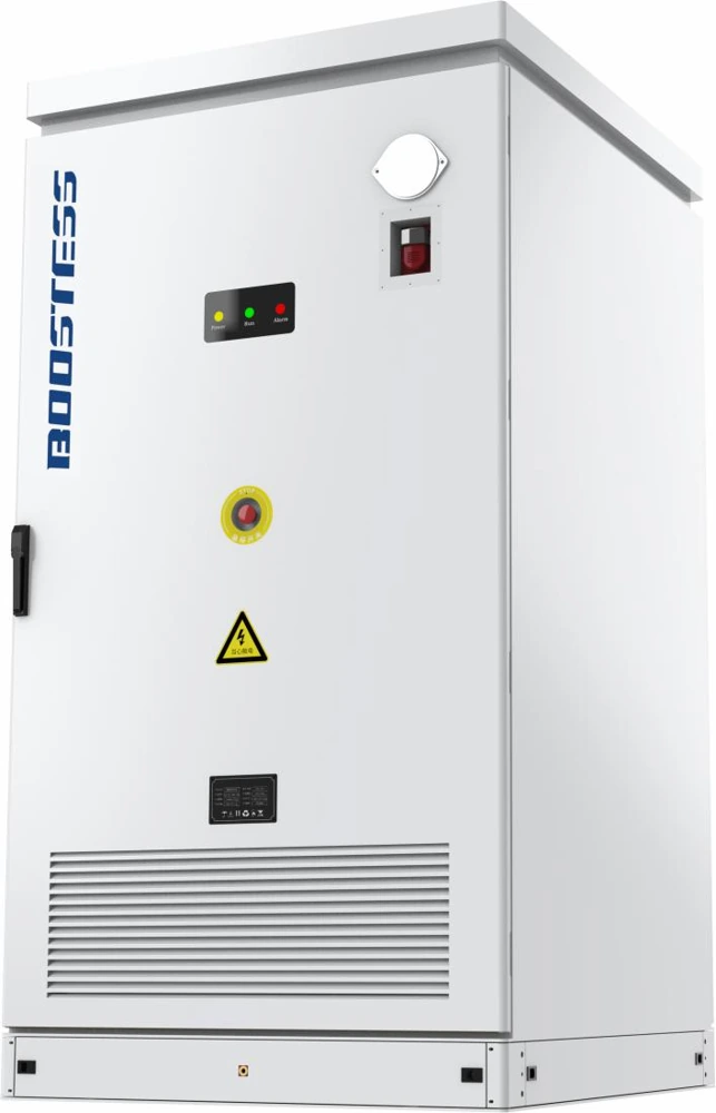
For equipment comparison, retain a second column showing required power during the entire event. The documented 125 kW / 261 kWh cabinet offers a different rated configuration from the 105 kW option, but neither single unit supplies the example’s 300 kW instantaneous gap at its nameplate rating. An averaged-demand strategy and a hard connection ceiling may therefore lead to different approved configurations. State the chosen objective beside each proposed model so that bidders cannot quietly change the problem being priced.
Make acceptance data resemble billing data
Agree the dataset before commissioning: connection energy, interval demand, battery power and energy, state of charge, commands, alarms and meter timestamps. The DOE BESS evaluation method uses metered time-series information for system assessment. For this project, the owner also needs the utility’s interval definition to verify the demand objective.
Choose events that distinguish competing control strategies. Include a short spike, a longer plateau, consecutive peaks, low available battery energy and charging recovery. Where the agreed test cannot safely occur during live production, use an approved simulated or controlled method and state that limitation in the report.
Define pass criteria separately for electrical and billing performance. The electrical criterion might address an agreed connection-power boundary. The billing criterion should use the actual demand calculation over the defined period. Avoid one ambiguous commitment to “reduce peaks,” which can mean either result.
Handover should include the tariff assumptions, controller settings and a change-review process. A new production line, revised shift or new meter configuration can invalidate the original operating model. Keep the demand worksheet with the site’s energy records so that staff can identify why performance has changed.
Questions the buyer should ask
Does a 500 kW spike require a 500 kW battery?
The answer depends on the objective, baseline load and event duration. A strict instantaneous ceiling can create a large power requirement. An averaged billing objective may need a different dispatch. Neither should be selected from the spike value alone.
Can a cabinet with two nominal hours of energy manage factory demand?
Possibly. Use the measured events, available AC power, usable energy and recharge schedule to assess it. A nominal duration ratio does not show whether repeated peaks or reserve restrictions leave enough support.
How can the owner verify a savings proposal?
Require a reproducible tariff calculation, measured load inputs and time-stamped dispatch results. Separate projected bill effects from witnessed technical performance. The strongest proposal shows which assumptions drive the result and how the owner can check them after handover.